案例解析：基因组组装

什么是基因组组装

基因组组装（Genome assembly）是使用测序方法将待测物种的基因组生成序列片段（即read），然后根据reads之间的重叠区域对片段进行拼接。首先，这些片段被拼接成较长的连续序列（contig），然后将contigs拼接成更长的允许包含空白序列（gap）的scaffolds。通过消除scaffolds的错误和gaps，我们可以将这些scaffolds定位到染色体上，从而得到高质量的全基因组序列。这个过程对于研究物种的基因组结构、功能基因挖掘、调控代谢网络构建以及物种进化分析等方面具有重要意义。

随着测序技术的进步和测序成本的降低，我们能够在短时间内获得大量的测序数据，然而基因组组装是一个复杂的过程，尤其是面临动植物等复杂且规模巨大的基因组的组装需要耗费大量的计算资源，因此，如何高效的分析和处理这些数据成为目前基因组学和生物信息学最亟待解决的问题。

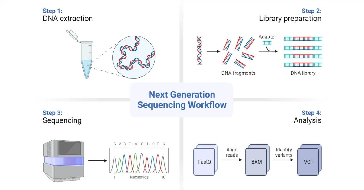
图1 DNA 测序流程图（引自：Next-Generation Sequencing (NGS)- Definition, Types (microbenotes.com)

基因组组装常见算法

基因组组装算法涉及多种方法，分为有参考基因组的组装和无参考的从头组装（de novo assembly），其中从头组装最常见的两个策略是基于德布鲁因图（De Bruijn graph）和Overlap-Layout-Consensus（OLC）的组装算法。

德布鲁因图（De Bruijn graph）

德布鲁因图是一种有向图，由节点和边构成，其要求是相邻两个节点的元素错开一个碱基。通过将测序得到的reads以k-mer方式排列，德布鲁因图可以帮助我们拼接成更长的Contig。例如，如果几条reads之间有overlap，那么就容易拼接成一个比较长的Contig。实际情况会更复杂，但我们通常保留主干路径，由主干路径组装成Contig1。

Overlap-Layout-Consensus（OLC）

OLC方法首先构建重叠图，然后将重叠图收束成Contig，最后选择每个Contig中最有可能的核苷酸序列。重叠图表示对于一些序列，前后有若干个碱基是一样的。多个reads片段可以构成重叠图。寻找最短的Contig序列，使得所有的reads都是该序列的子集，通常采用贪心算法实现。

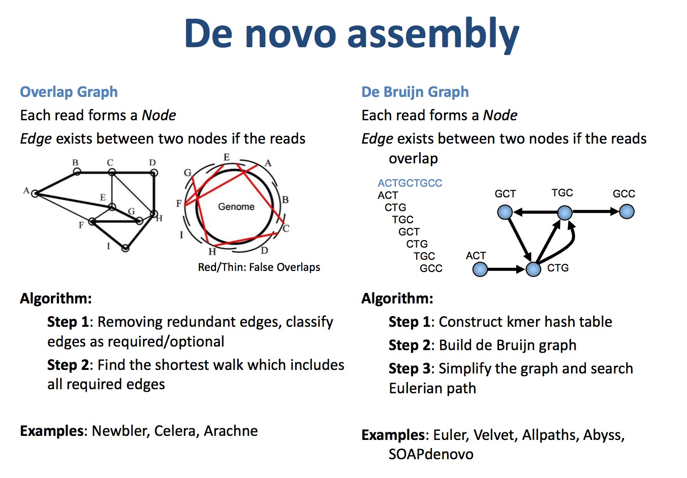
图2 OLC (左)和 DBG 算法示意图（右）(引用自：https://qinqianshan.com/bioinformatics/bin/olc-dbg/)

应用量子计算解决基因组组装问题

问题转化

高质量的基因组装需要较高深度的测序才能满足要求，对于完整的人类基因组组装，通常建议的覆盖度在30x以上。以三代测序（如PacBio和Oxford Nanopore等）用于人类基因组组装为例，通常每个read可以达到几千到几万个碱基，覆盖30x的情况下，可能需要的reads数量在几百万到几千万不等。如此庞大的reads组装在计算重叠图(overlap graph)时通常面临巨大的计算复杂度和算力需求，因此经典计算通常引入重叠过滤、动态规划等方法来降低计算复杂度，如果组装高质量的基因组则需要耗费大量时间，这里我们引入量子算法来加速这一过程。

OLC算法中最关键的一步是通过构建重叠图来确定不同reads间的位置关系，这一步可以转换成组合优化问题的旅行商问题（Traveling Salesman Problem，TSP）。其中不同reads表示不同的城市结点，reads间的重叠长度作为结点间的权重，目标是将所有的reads按照它们之间的重叠长度进行排序，并尝试将它们组装成一个总体重叠长度最长的序列，如图三所示。

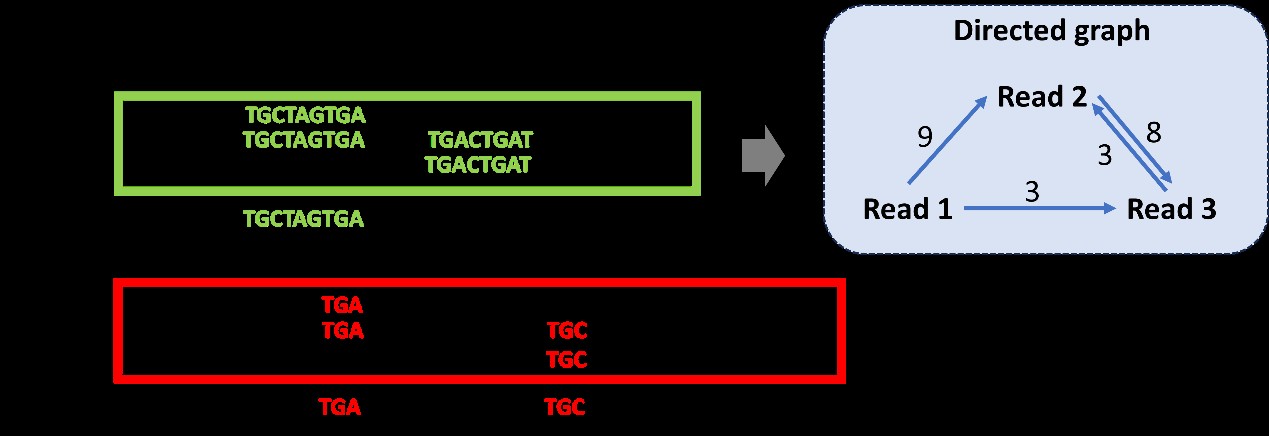
图3 测序reads组装转换为有向图模型

建模步骤

1）变量定义

在该模型中我们将所有reads设为节点，节点的边的权重为两个reads按顺序前后拼接的重叠长度，这样就构成一个带权有向图，目标为寻找总体重叠长度最长的reads序列则转化为寻找权重最大的哈密顿回路。将带权有向图用邻接矩阵表示： $t s p A d j M a t r i x_{i j}$ ，元素的下标表示 $R e a d s_{i}$ 在前、 $R e a d s_{j}$ 在后的拼接重叠长度。如果重叠长度不大于阈值，或者 $𝑖 = 𝑗$ ，则 $t s p A d j M a t r i x_{i j} = 0$ 。决策变量 $R e a d s_{i j}$ 取值为 ${0, 1}$ ，1表示 $R e a d s_{i}$ 排在第 $j$ 个位置，否则为0。

我们想得最大重叠长度，目标函数可写成：

H_{o b j} = δ \sum_{(u, v) \in E} t s p A d j M a t r i x_{u, v} (\sum_{j = 0}^{n - 1} R e a d s_{u, j} R e a d s_{v, j + 1} + R e a d s_{u, n - 1} R e a d s_{v, 0})

2）约束条件处理

一个reads必须而且只能出现在序列中的一个位置，$\sum*{j = 1}^{n}Reads_Sort*{ij}=1$，

序列中的一个位置必须而且只能被一个reads占用，$\sum*{i = 1}^{n}Reads_Sort*{ij}=1$，

将以上两个约束写成QUBO形式，有：

H_{s e q_c o n} = γ \sum_{i = 0}^{N - 1} (\sum_{j = 0}^{N - 1} R e a d s_{S o r t_{i j}} - 1)^{2}

H_{n o d e_c o n} = γ \sum_{j = 0}^{N - 1} (\sum_{i = 0}^{N - 1} R e a d s_{S o r t_{i j}} - 1)^{2}

3) QUBO 模型构建

如此，由以上的约束条件，我们可以构建一个遍历所有的点的路径的模型（又称哈密尔顿环）：

H = - H_{o b j} + H_{s e q_c o n} + H_{n o d e_c o n}

优化目标是求 H 的最小值。

４）使用Kaiwu SDK实现用Solver直接对QUBO Model进行求解

python

"""
TSP-based DNA sequence assembly with reference answer generation.
"""

import random

import numpy as np
import kaiwu as kw


np.set_printoptions(linewidth=1000)
SEED = 0


class DNAReconstruction:
    """
    Build a QUBO model for DNA sequence assembly using TSP transformation.
    """

    def __init__(self) -> None:
        self.reads = []  # Sequence reads
        self.cutpoint = []  # Cut points
        self.reads_sort = None
        self.answer = None
        self.qubo_model = None
        self.path_cost = None
        self.ham_cycle = None

    @staticmethod
    def _align_core(read1, read2, max_mismatch, cut_off):
        """
        Core alignment logic shared by align and aligncycle methods.
        Returns the shift value and mismatch count if alignment is successful, otherwise returns None.
        """
        l1 = len(read1)
        for shift in range(0, l1 - cut_off):
            mismatch = 0  # Number of mismatched bases
            r2i = 0
            for r1i in range(shift, l1):
                if read1[r1i] != read2[r2i]:
                    mismatch += 1  # Increment mismatch count
                if r2i < len(read2) - 1:
                    r2i += 1
                else:
                    break

                if mismatch > max_mismatch:  # If mismatches exceed tolerance, break out
                    break

            if mismatch <= max_mismatch:  # If mismatches are within tolerance
                return shift, mismatch  # Return the shift value and mismatch count

        return None  # No valid alignment found

    @staticmethod
    def align(read1, read2, max_mismatch, cut_off):
        """
        Overlap module, Read1 is the head and Read2 is the tail for alignment, returning the overlap length.
        """
        result = DNAReconstruction._align_core(read1, read2, max_mismatch, cut_off)
        if result:
            shift, _ = result
            return min(len(read1) - shift, len(read2))
        return 0

    @staticmethod
    def aligncycle(read1, read2, max_mismatch, cut_off):
        """
        Overlap module, Read1 is the head and Read2 is the tail for alignment, returning the initial position.
        """
        result = DNAReconstruction._align_core(read1, read2, max_mismatch, cut_off)
        if result:
            shift, _ = result
            return len(read1) - shift
        return 0

    def shot_gun(self, gene_ref, reads_number):
        """
        Given a gene sequence Gene_ref, replicate it reads_number times,
         connecting the ends, then randomly cut each loop in half
        """
        self.reads = []  # Sequence reads
        self.cutpoint = []  # Cut points
        n = len(gene_ref)

        for _ in range(0, reads_number):
            # Randomly cut the n-length gene sequence into two segments,
            # resulting in 2n reads
            cut_1 = random.randint(0, len(gene_ref) - 1)
            cut_2 = (cut_1 + round(len(gene_ref) / 2) + random.randint(-40, 40)) % n
            # Randomly cut the gene sequence at two points,
            # making the segments approximately equal in length with a ±10% variation
            gene_cut_1 = min(cut_1, cut_2)
            gene_cut_2 = max(cut_1, cut_2)
            self.cutpoint.append(gene_cut_1)
            self.cutpoint.append(gene_cut_2)
            self.reads.append(gene_ref[gene_cut_1 : gene_cut_2 - 1])  # One segment
            self.reads.append(
                gene_ref[gene_cut_2 - 1 :] + gene_ref[0:gene_cut_1]
            )  # The other segment

    def merge_seq(self, dna_sort):
        """
        Consensus module, assemble DNA according to the sorting order.
        Given a sequence, return the reads assembled in that order.
        """
        merge = self.reads[dna_sort[0]]  # Reconstruct the gene sequence
        n = len(self.reads)
        sum_overlap = 0  # Total overlap length
        r1i = 0
        r2i = 0

        # Connect gene fragments in the order of the solution, starting from the 0th and going to the n-1th
        while r2i < (n - 1):
            r2i += 1
            overlap = self.align(
                self.reads[dna_sort[r1i]], self.reads[dna_sort[r2i]], 0, 0
            )

            overlap1 = self.align(
                self.reads[dna_sort[r2i - 1]], self.reads[dna_sort[r2i]], 0, 0
            )

            sum_overlap = overlap1 + sum_overlap
            # If overlap length is greater than R2 length, R1 completely covers R2,
            # skip fusion. R1 stays, and R2 moves to the next.
            if len(self.reads[dna_sort[r2i]]) > overlap:
                merge = merge + self.reads[dna_sort[r2i]][overlap:]
                r1i = r2i

        # Then connect the current longest tail with the 0th
        overlap = self.aligncycle(
            self.reads[dna_sort[n - 1 - r2i + r1i]], self.reads[dna_sort[0]], 0, 0
        )

        if overlap != 0:
            merge = merge[:-overlap]
        if len(self.reads[dna_sort[0]]) > overlap:
            sum_overlap = overlap + sum_overlap
        else:
            sum_overlap = len(self.reads[dna_sort[0]]) + sum_overlap
        return [merge, sum_overlap]

    def prepare_model(self, gene_ref, reads_number, constraint, max_mismatch, cut_off):
        """
        Convert DNA sequencing reads into a TSP adjacency matrix,
         where the edge weights are the overlaps,
         and the direction of the edge is row index → column index
        """
        self.shot_gun(gene_ref, reads_number)
        n = len(self.reads)
        tsp_adj_matrix = np.zeros((n, n))
        for r1 in range(0, n):
            for r2 in range(0, n):
                if r1 != r2:
                    tsp_adj_matrix[r1][r2] = self.align(
                        self.reads[r1], self.reads[r2], max_mismatch, cut_off
                    )

        # Create the QUBO variable matrix.
        # The variable Reads_Sort(i,j) means that the i-th gene read is sorted in the j-th position
        self.reads_sort = kw.core.ndarray((n, n), "Reads_Sort", kw.core.Binary)

        w = tsp_adj_matrix

        # Get the set of edges and non-edges
        edges = [(u, v) for u in range(n) for v in range(n) if w[u, v] != 0]

        # Read constraints: each read should belong to only one position
        sequence_cons = kw.core.quicksum(
            [
                (1 - kw.core.quicksum([self.reads_sort[v, j] for j in range(n)])) ** 2
                for v in range(n)
            ]
        )

        # Position constraints: each position should have only one read
        node_cons = kw.core.quicksum(
            [
                (1 - kw.core.quicksum([self.reads_sort[v, j] for v in range(n)])) ** 2
                for j in range(n)
            ]
        )

        # Hamiltonian cycle constraint, removing edge constraints
        self.ham_cycle = sequence_cons + node_cons

        # Total COST is the sum of overlap lengths;
        # since the total length of DNA fragments should be minimized,
        # COST should be maximized, so the negative sign is taken in the objective function
        self.path_cost = -kw.core.quicksum(
            [
                w[u, v]
                * (
                    kw.core.quicksum(
                        [
                            self.reads_sort[u, j] * self.reads_sort[v, j + 1]
                            for j in range(n - 1)
                        ]
                    )
                    + self.reads_sort[u, n - 1] * self.reads_sort[v, 0]
                )
                for u, v in edges
            ]
        )

        qubo_model = kw.core.QuboModel()
        obj = constraint * self.ham_cycle + self.path_cost
        qubo_model.set_objective(obj)

        self.qubo_model = qubo_model

    def print_answer(self):
        """
        First restore the reference answer as an IS matrix,
        then add the spin term to get the reference answer's solution vector Answer_vec,
        and the reference answer provides other information
        """

        self.answer = np.argsort(self.cutpoint)  # Reference answer
        n = len(self.reads)  # Number of reads

        mat_answer = np.zeros((n, n), dtype=int)
        for i, x in enumerate(self.answer):
            mat_answer[i, x] = 1
        return mat_answer


if __name__ == "__main__":
    dna_reconstruction = DNAReconstruction()
    GENE_REF = (
        "ATGGCTGCTAGGCTGTGCTGCCAACTGGATCCTGCGCGGGACGTCCTTTGTTTA"
        "CGTCCCGTCGGCGCTGAATCCTGCGGACGACCCTTCTCGGGGTCGCTTGGGACT"
        "CTCTCGTCCCCTTCTCCGTCTGCCGTTCCGACCGACCACGGGGCGCACCTCTCT"
    )
    # Prepare the model, testing reads_number with 7, 8, 9, and 10
    # Duplicate the DNA sequence into reads_number copies, connect the ends,
    # and randomly cut each circle into two halves
    READS_NUMBER = 3
    # max_mismatch is the allowed mismatch in DNA alignment; exceeding it means the reads are not adjacent
    MAX_MISMATCH = 0
    # cut_off is the minimum overlap length threshold; if the overlap length between two reads
    # does not reach the threshold, it is set to 0
    CUT_OFF = 3
    # The penalty coefficient for the Hamiltonian constraint in the final objective function
    CONSTRAINT = 200

    """
    Amplify the DNA sequence and randomly cut it into fragments using the shotgun method.
    Then sequence to obtain reads (this does not account for sequencing errors; fragments are directly used as reads).
    Store these reads as a weighted directed graph based on overlap length, and convert it into a TSP-like QUBO model.
    Based on the standard assembly order of the reference gene, provide the solution vector, Hamiltonian,
    and path length Hamiltonian for reference.
    """
    dna_reconstruction.prepare_model(
        GENE_REF, READS_NUMBER, CONSTRAINT, MAX_MISMATCH, CUT_OFF
    )

    solver = kw.classical.SimulatedAnnealingOptimizer(
        initial_temperature=10000,
        alpha=0.9,
        cutoff_temperature=0.01,
        iterations_per_t=200,
        size_limit=100,
    )
    sol_dict, qubo_val = solver.solve_qubo(dna_reconstruction.qubo_model)

    # Substitute the spin vector and obtain the result dictionary
    ham_val = kw.core.get_val(dna_reconstruction.ham_cycle, sol_dict)

    print(f"ham_cycle: {ham_val}")

    # Calculate the path length using path_cost
    path_val = kw.core.get_val(dna_reconstruction.path_cost, sol_dict)
    print(f"path_cost: {path_val}")

量子计算与经典方法的效果对比

我们比较了在不同问题规模下（reads数分别为7、8、9、10）SPQC量子真机和传统求解器Simulated Annealing、Tabu Search的求解时间。对比发现，在同等规模问题上，SPQC真机的求解时间要远少于Simulated Annealing、Tabu Search（左图）。同时，随着问题规模增大，SPQC真机求解时间相较于Simulated Annealing、Tabu Search更加稳定（右）。

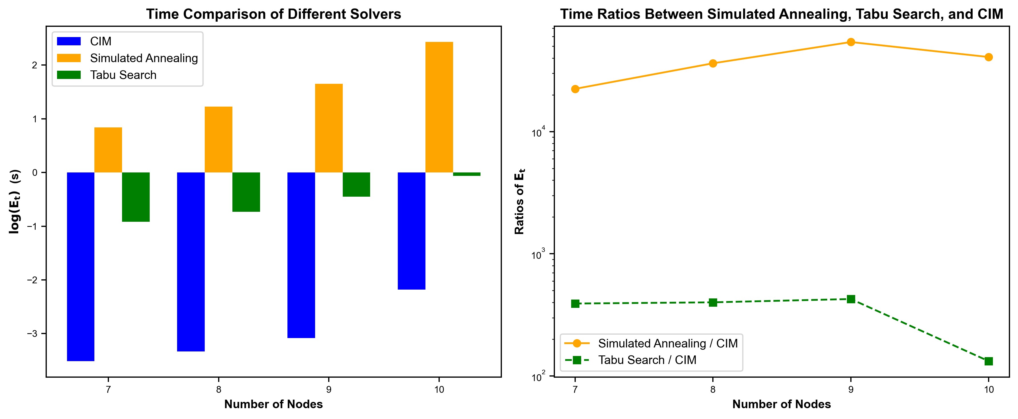
图4 不同问题规模下（reads数分别为7、8、9、10）SPQC真机和传统求解器Simulated Annealing、Tabu Search的求解时间对比

以reads 数为7的问题求解为例，我们可以发现量子真机相较于SA算法，其哈密顿量能快速下降以求得最优解。

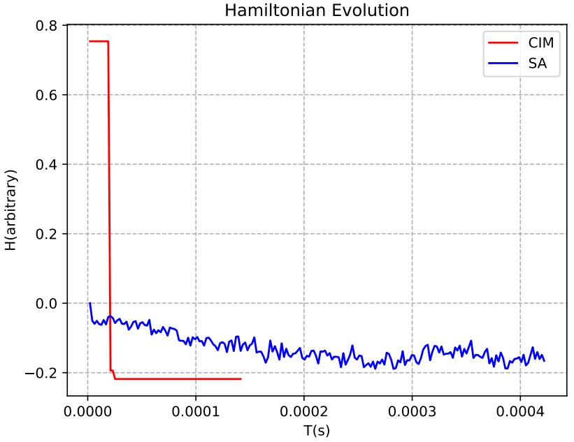
图5 Reads数为7时的量子真机（红线）、SA（蓝线）哈密顿量演化图

案例解析：基因组组装 ​

什么是基因组组装 ​

基因组组装常见算法 ​

应用量子计算解决基因组组装问题 ​

问题转化 ​

建模步骤 ​

量子计算与经典方法的效果对比 ​